Electronic Pages

Die Homepage der Familie Beis

Motion and direction detection with a dual-channel radar sensor

- An experimental setup that delivers interesting results -

( Deutsche Version: Bewegungs- und Richtungserkennung mit einem zweikanaligen Radar-Sensor)

Contents

Foreword

It was pure curiosity that prompted me to buy a Rader sensor and see what could be achieved with it. There was no other goal than to satisfy my curiosity. But the test results were so interesting that at least this article resulted from them.

There was a question in a forum about a technology to check whether a bedridden person was still showing signs of life. I think that the use of such radar sensors would be quite ideal for this in various aspects.

The radar sensor

Many different radar sensors are offered on the relevant Chinese trading platform. I was interested in the simple ones with analog outputs because I wanted to carry out my experiments on a breadboard and not in firmware. They are supplied with 5 V.

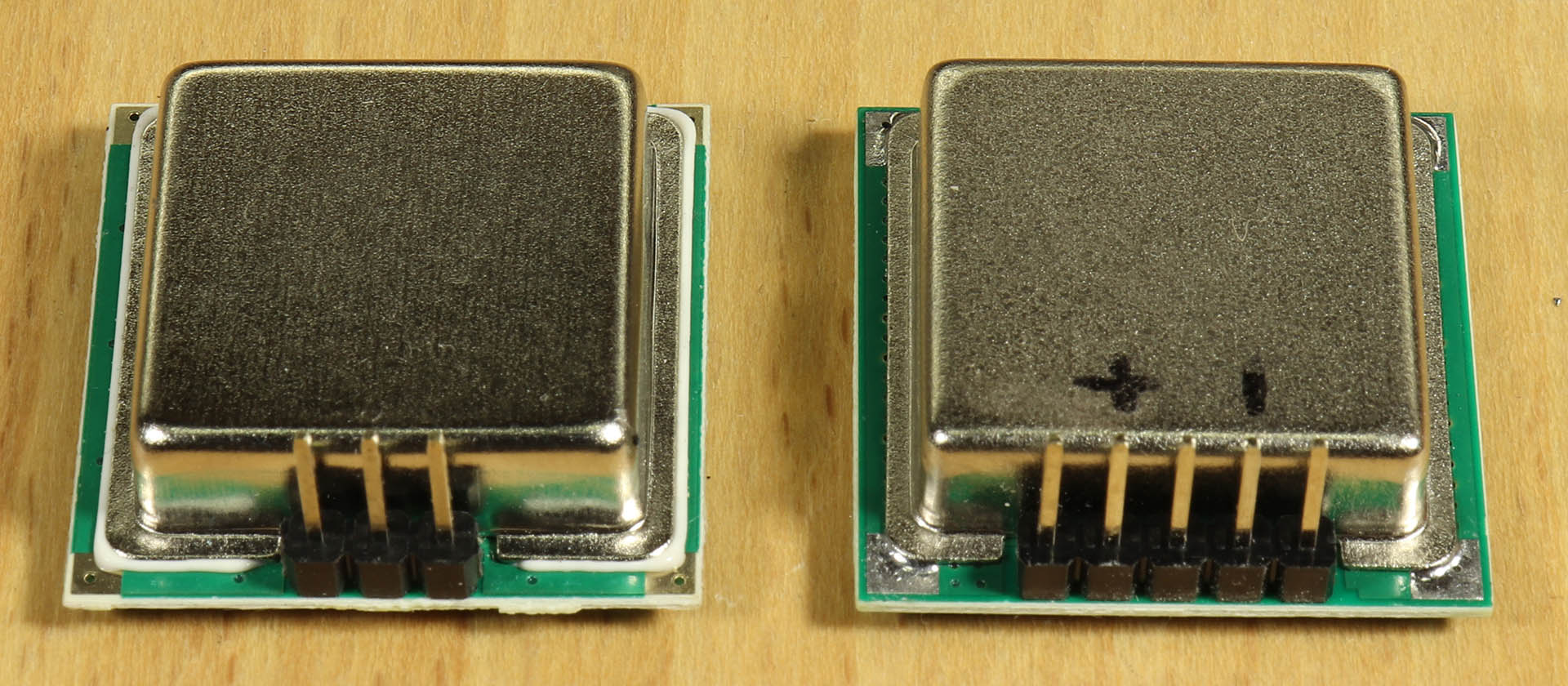
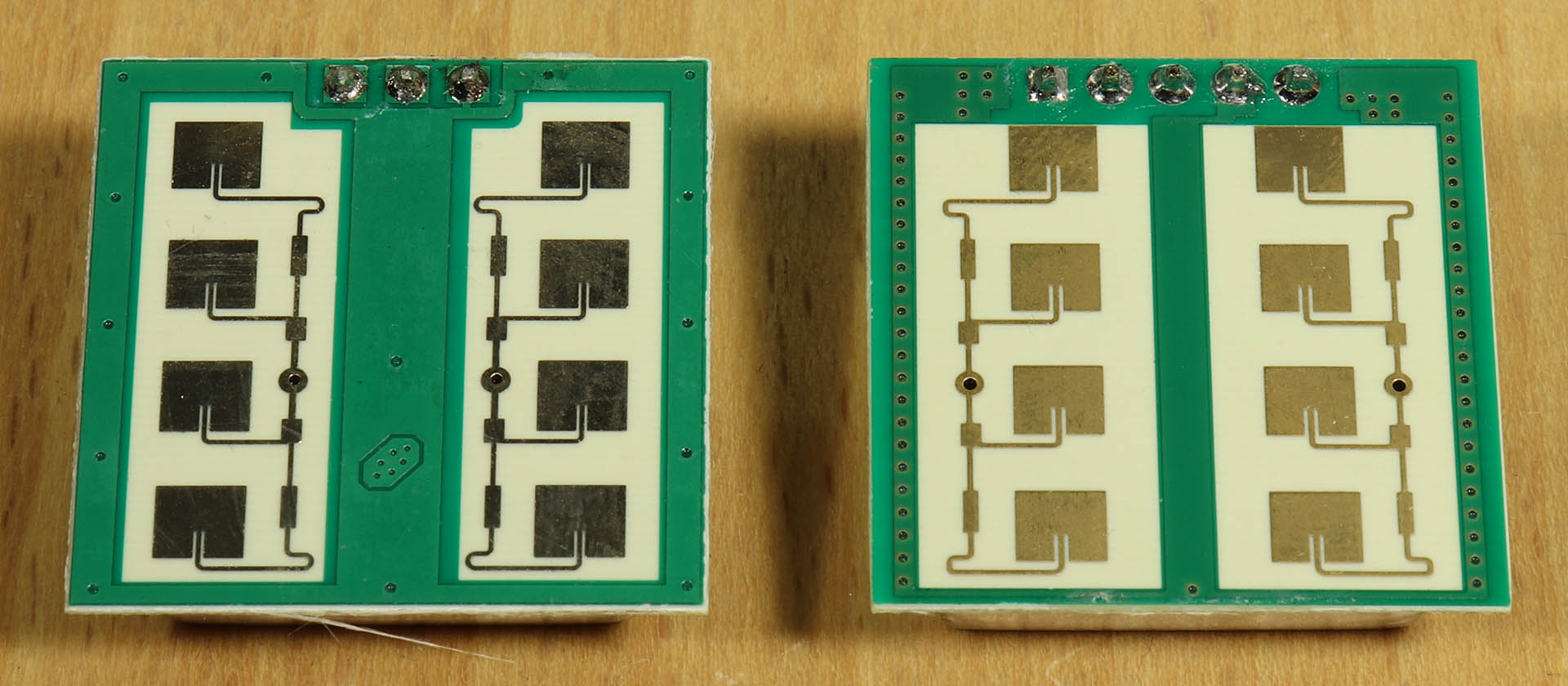
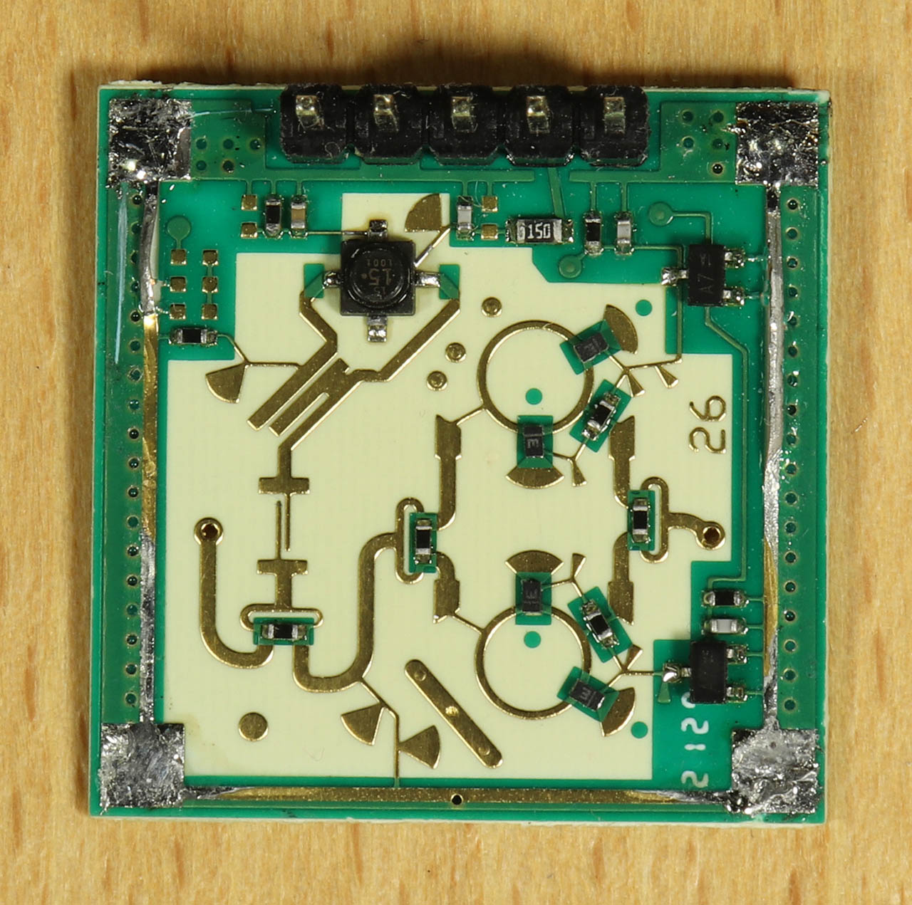
There are single-channel (3-pin) and dual-channel (5-pin, only 4 connected) sensors. 3^rd picture: The two-channel sensor inside.

The single-channel sensor

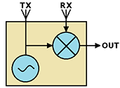
In principle, all (or at least very many) of these sensors transmit an RF carrier at ~24 GHz. The reflected signal is received by a second antenna arrangement and demodulated by multiplication with the carrier and output as an analog signal. This analog signal can be both positive and negative as well as very small and must be amplified accordingly.

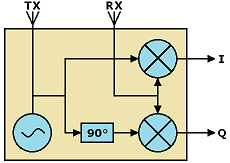The dual-channel sensor

In addition to the simple single-channel sensors, there are also dual-channel sensors. With these, the received signal is not only demodulated with the carrier directly, but also with the carrier phase-shifted by 90° and output as a second analog signal. As a result, the two output signals are also phase-shifted by 90° during movements, so that one phase runs 90° ahead or behind when the object approaches and the other phase runs 90° ahead or behind when the object moves away.

The two outputs or output signals are usually called I and Q.

I was particularly interested in the possibilities offered by the two-channel sensor. However, such a sensor costs many times more than a single-channel sensor. And to make matters worse, I had destroyed a sensor through carelessness, so it cost me twice as much. But in return I can also offer an interior shot of the defective sensor.

Attention: At least with the two-channel AM182 sensors that I have, there are two different pin assignments! They are called AM182-I and AM182-R. I could only find out which one I had received by measuring which pin is the ground. I have version AM182-R.

Similarities, experiences

The technical data is not available for all, but for some offers.

The wavelength of 24 GHz is approx. 12.5 mm, so that a complete cycle with maximum and minimum should theoretically occur every 6.25 mm when the distance changes. If, for example, a pedestrian moves towards the sensor at 3.6 km/h = 1 m/s, there would be 160 cycles within one second. Ideally, this would result in a sinusoidal signal with a frequency of 160 Hz.

But in practice it is somewhat more because the object has a considerable extension. Reflections reach the sensor via paths of different lengths, which result in different relative speeds. In addition, the overlapping partial reflections increase and decrease, so that the signal ultimately deviates significantly from the ideal.

The output impedance is relatively low at a few 10 Ω. The output voltages are around 0 V and are not DC-free. This means that, depending on the distance of the object, negative voltages can also come out of the outputs permanently. These can be more than ±100 mV for objects very close to the sensor. The inherent noise is approx. 10 µVpp (500 Hz band-limited measurement), but there is hardly a situation in which changes in the environment do not generate higher signals.

Example, screenshot on the right (gain 60 dB, 500 Hz bandwidth): If I sit as still as possible in front of the sensor at a distance of 2 m and hold my breath, my heartbeat of up to 100 µVpp can be clearly seen in this screenshot. However, it is not always so clear to see, because the movement is minimal, and if the reflected and demodulated phase happens to be at a maximum or minimum, there is practically no signal, at least on one channel. However, it should be optimal on the other channel in the 0-pass, although this is not guaranteed.

24 GHz does not penetrate many materials. I haven't done any detailed research or looked for information on this. But I have gathered at least a little experience. Plastics such as ABS, PS and PMMA (acrylic glass) and thick cardboard have almost no attenuation, while a simple pane of glass has an estimated attenuation of 50%. Almost(?) nothing passes through my triple-glazed window pane, but through its plastic frame, which obviously also absorbs sound, I can clearly see cars driving past at a distance of 5 m, but not, or at best only vaguely, people or cyclists, for example. Only a little penetrates through my wooden room door. The brickwork shields it completely.

Signal evaluation

Of course, the output signals must first be amplified considerably for any kind of evaluation. I have chosen two-stage amplification of approx. 30 dB each with band limiting in each stage at 500 Hz. This means that the amplifier is not overdriven even with relatively strong signals (i.e. close objects) that occur in practice. With a single-channel sensor, the AC signal from the amplifier would now be rectified with an analog circuit or a µC and displayed as movement.

With a two-channel sensor, the direction of the movement can also be detected by comparing the phase of the I/Q signals. Depending on which of the two phases is leading or lagging, approaching or moving away is then displayed. This could also be realized very well with a µC, especially if further evaluations of the signal are to take place. However, I already had the preamplifier on the breadboard, and an attempt to evaluate the direction on the breadboard was much easier, at least for me. It was also easier to observe with the oscilloscope, so in the end I stuck with the analog solution.

I would like to mention in advance that after the first attempts on the breadboard, I had little hope that the direction detection could work reliably, because the signals from the I/Q outputs do not look nearly as ideal in practice as one might expect. However, I was pleasantly surprised at how well and reliably it worked on the final setup.

Circuit description

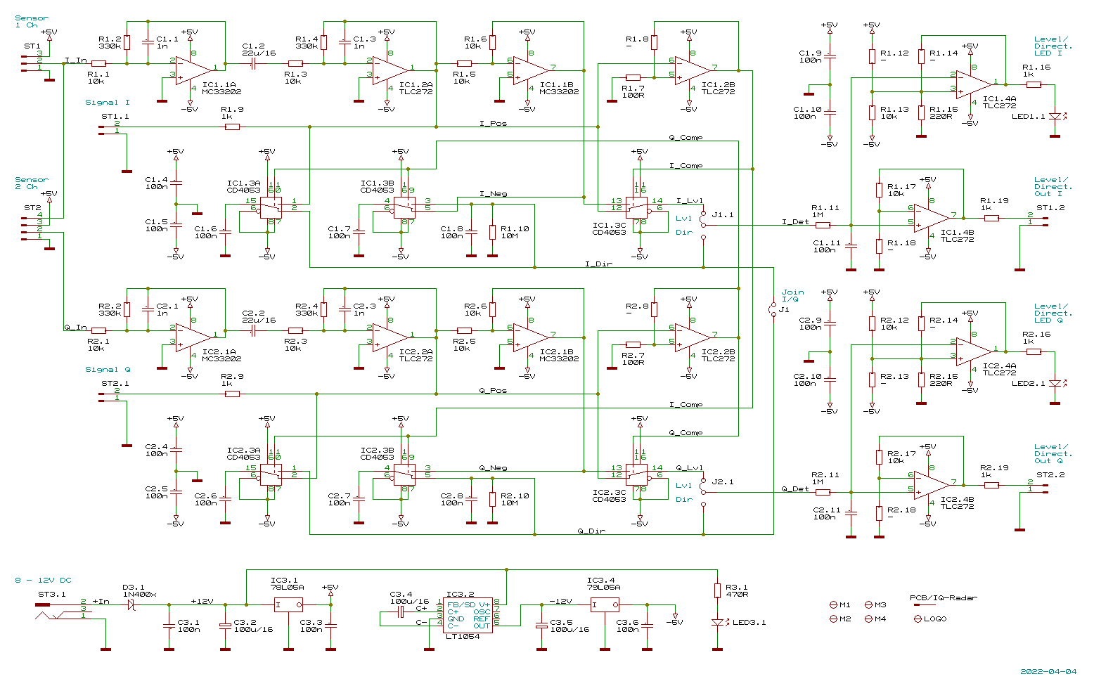There is a 2-stage preamplifier for each channel (channel 1: IC1.1A and IC1.2A). The second stage is AC-coupled and equipped with a J-FET op-amp so that its output voltage does not have a greater DC offset than that of the TLC272 itself. This is important for the following evaluation.

Direction detection

The amplified I and Q signals are also required in inverted form for direction detection (IC1.1B), as is detection for the 0 passage of the signal with a comparator (IC1.2B). As already mentioned, IC1.2A must be a J-FET op-amp, and IC1.2B must be able to work as a comparator, i.e. tolerate large differential input voltages. Most op-amps cannot do this, but the TLC272 can. IC1.1 is less critical, only the rail-to-rail I/O property and the lower noise at low frequencies of the MC33202 are welcome.

In principle, one signal (e.g. I) would have to be multiplied by the 90° shifted signal of the other channel (e.g. Q) to detect the direction. However, this is not possible in practice, as only fixed frequencies can be rotated in a defined phase. Here, however, there are very broadband signals, from less than 1 Hz to several 100 Hz. So this is not possible.

Track-and-Hold, Sample-and-Hold

To solve the task, the voltage of the other signal (e.g. Q) is determined at the same moment when one signal (e.g. I) passes through 0. Depending on the direction of movement, it is positive or negative. The level of the voltage naturally depends on the size and distance of the object. I have realized the determination of the voltage of one channel at the moment of the 0-crossing of the other channel with a (resp. 4) track-and-hold circuit(s).

Example: The voltage at capacitor C2.6 follows the signal Q_Pos as long as the switching signal I_Comp is low, i.e. while the signal I_Pos is positive ("tracking"). If signal I_pos changes polarity, which is ideally the case at the maximum of signal Q_Pos, there is a charge equalization between C2.6 and C2.8 (signal Q_Dir). This voltage can rise or fall. Both together result in a kind of sample-and-hold circuit.

Of course, the other half-wave of the signal Q is also taken into account. For this purpose, the signal Q_Neg is "tracked" with C2.7 and IC2.3 and its charge is transferred to C2.8 (signal Q_Dir) or combined with it at the other phase of signal I or I_Comp. Because Q_Neg is tracked, at this moment it has the same polarity as that of Q_Pos.

And of course, the voltage of channel Q is not only sampled with the phase of channel I, but also vice versa. If this were not inverted again, the signal Q_Dir would be inverse to I_Dir. The repeated inversion is the result of swapping the multiplexer connections 1/2 and 3/5 on IC2.3. The signals Q_Dir and I_Dir can now be connected to each other (jumper Join I/Q) and result in a common signal that should be of better quality than each individual signal.

It may also be clearer as a table. The sequence of events in this table would correspond to one direction of movement, the reverse sequence to the other direction of movement:

In principle, 74HC4053 would also be suitable for the multiplexers instead of CD4053, but I wanted to reduce the peak currents with the higher internal resistances of the CD4053. However, the resulting time constants of approx. 15 µs remain sufficiently small.

Detection of the signal strength

With single-channel sensors, you can or must of course limit yourself to evaluating the signal amplitude for simple motion detection. Because a multiplexer was still free, polarity detection using a comparator and inverting of the sensor signal was already available, the multiplexer IC1.3 is used to rectify the sensor signal. The signal level ("Level") is then formed in the low-pass filter R1.11 / C1.11.

Two independent, single-channel sensors can be connected and evaluated.

Output and signaling

Signal level or direction display is selected with the Lvl/Dir jumpers. IC1.4 could also amplify the signals, but it is probably better to leave it at a 1:1 buffer. IC1.4A can be wired as a comparator with hysteresis (= Schmitt trigger) or without hysteresis, as well as with different switching thresholds. I have omitted the hysteresis. I have selected the thresholds for direction detection at approx. -100 mV (approach) and +100 mV (move away). For the latter comparator, which should light up the LED at voltages of > 100 mV but works inverted, the LED must be fitted with reversed polarity(!)

Practical assembly

I had already gained a lot of experience from the experiments on the breadboard, but I was still unsure about a number of details. This applied in particular to the final dimensioning. That's why I opted for a circuit board with THT components, where I could make all components (except the power supply) pluggable. In the end, not many of the originally planned dimensions changed, but a number of the planned resistors turned out to be superfluous. But of all things, I had to replace the only permanently soldered components, the electrolytic capacitors C1.2 and C2.2, with bipolar ones.

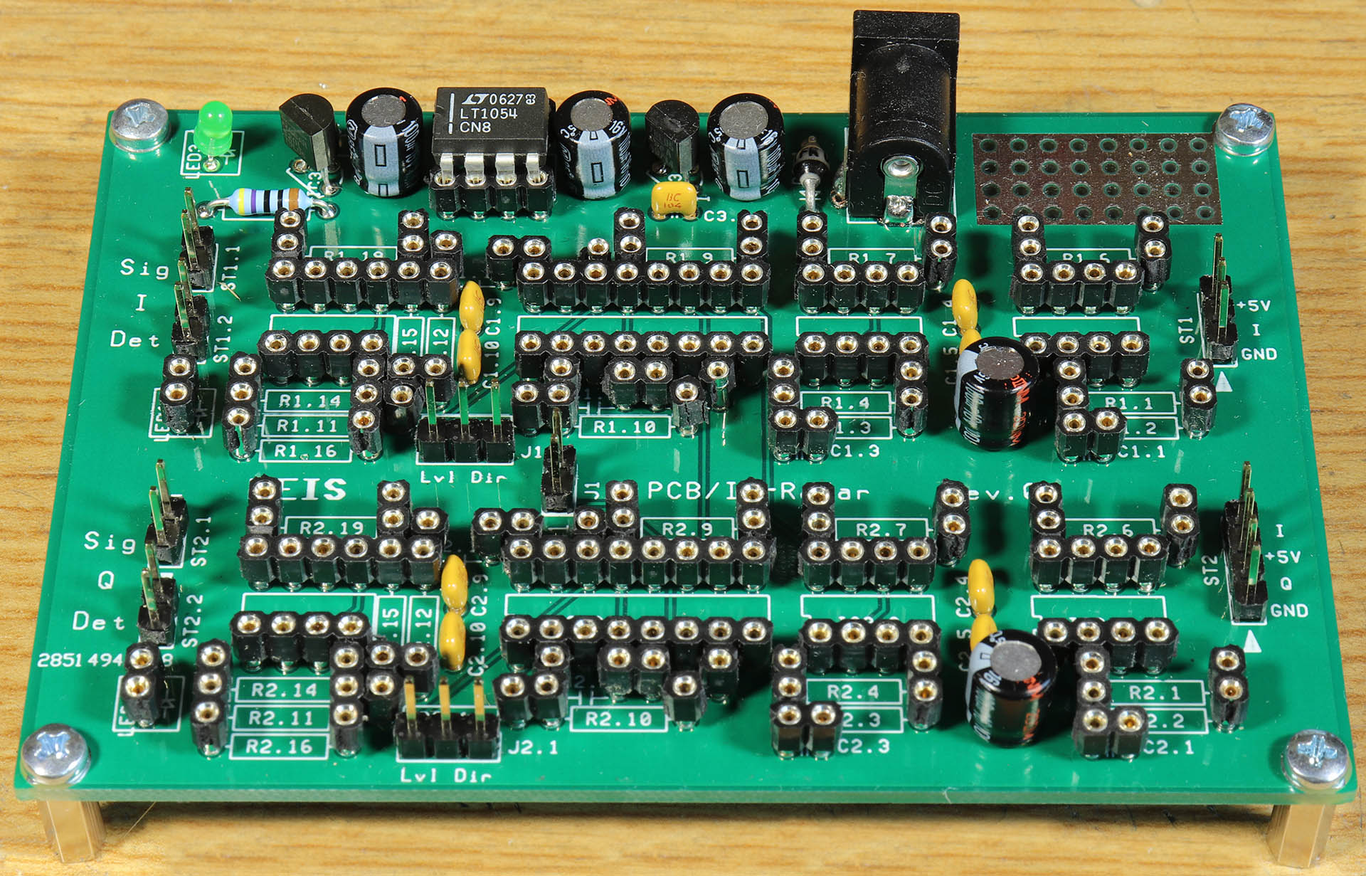
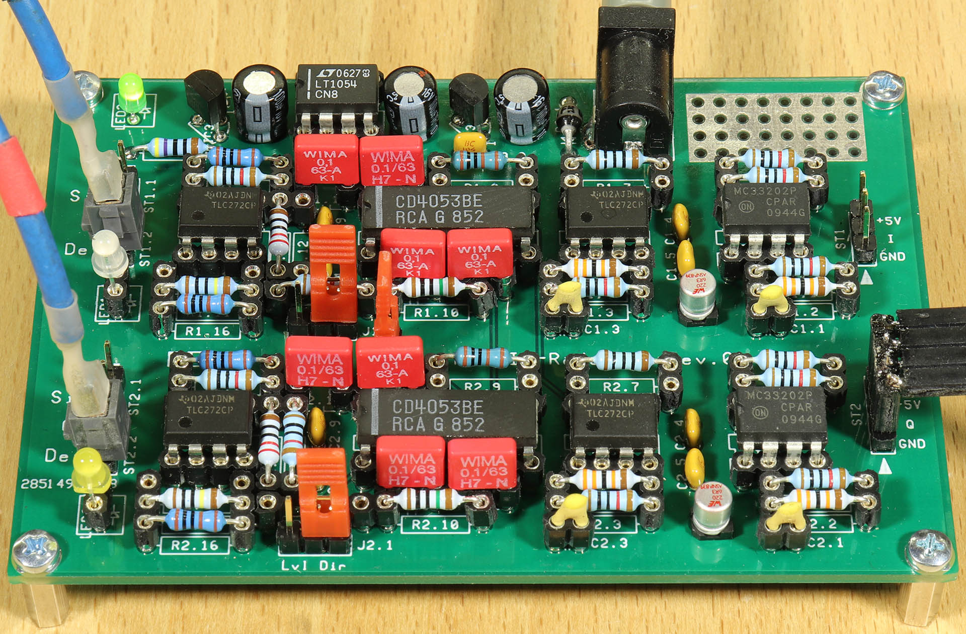
Apart from that, the layout was flawless (unusual...), but I would perhaps add a 4-pole pin header including the necessary components to be able to connect a µC for digital evaluation directly, or perhaps a switching output for external signalling devices. There is still a bit of space in the breadboard area. But I don't really have any further plans for this project.

A few more screenshots

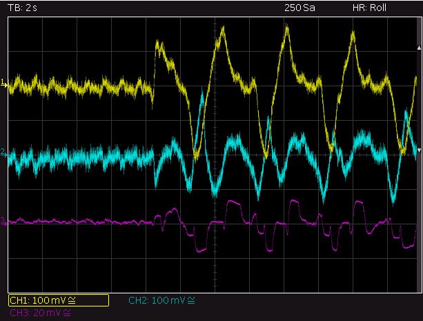
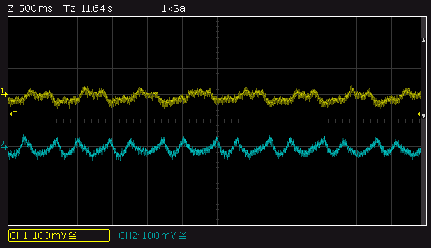
The pictures show, from top to bottom, the signals I, Q and Direction from the direction evaluation. Both pictures were taken from about 2 meters away from me, sitting on the office chair, as an "object" for the movement.

For the first image, I first sat very still and held my breath. As in the screenshot above, you can see the heartbeat. Then I breathed normally. With such small movements, the direction of movement can hardly be recognized, but nevertheless: You can see that the directional signal changes only slightly more often than perhaps 1 time per second. This is no wonder: with a breathing cycle lasting approx. 4 seconds, there are only a total of 4 0-passes of the I and Q signals during which the directional evaluation takes place. The fact that the signals are far from ideal and also result in more 0-passages does little to change the fact that the result makes perfect sense.

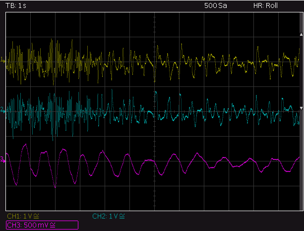
In the second image, I first rocked my upper body back and forth quickly and with a large amplitude while sitting on the chair, then slowly with a low amplitude. The rocking frequency is approximately the same in both cases, only the speed of movement is different. You can see in the I and Q signal that several superimposition phases are passed through due to the greater distance, whereas with the low amplitude there is hardly more than one. The direction is still recognized correctly.

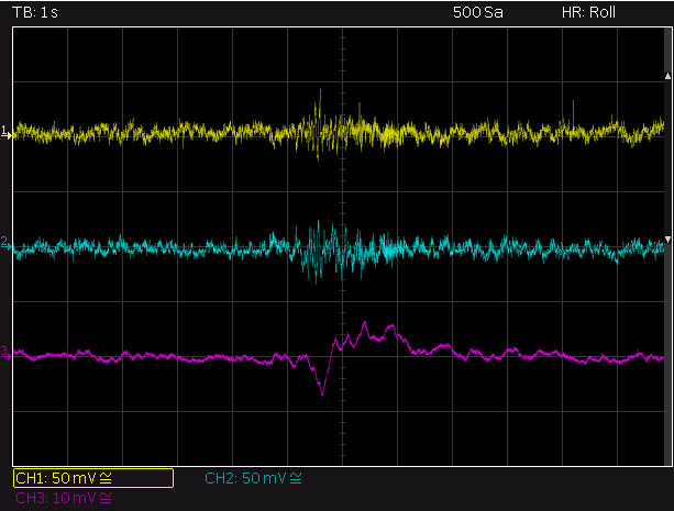
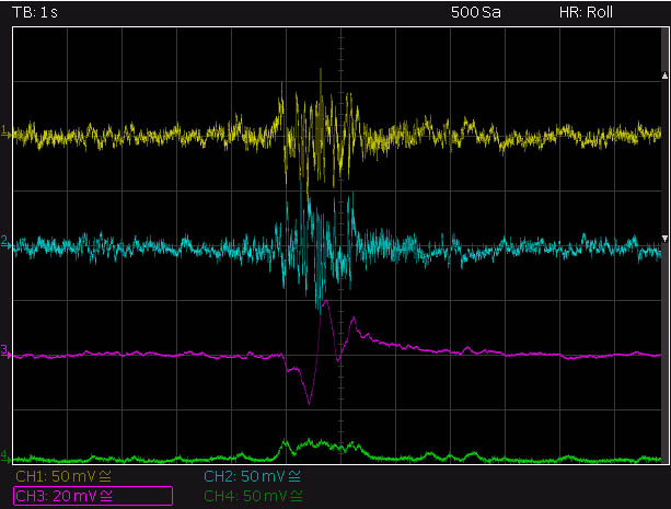
Here, the first image was taken by a car driving past at a distance of approx. 5 m, with the sensor in my room positioned directly behind the plastic frame of the window. The speed is decreasing from an estimated 20 to 5 km/h. The signals are weak, not much stronger than the noise, but the direction detection still provides a relatively clear signal: first the car approaches quickly and then moves away more slowly.

The second image shows a similar situation, only the vehicle is much larger, comparable to a large van. The vehicle braked to a halt just a few meters after passing, i.e. still within the sensor's detection range. The direction detection is clear, but I can't explain the dip after the 1^st positive maximum. A video would have been helpful. It should be noted that the scaling here is 20 instead of 10 mV/sec previously. The 4^th signal shows the level of the I signal (I_Lvl)