Electronic Pages

Die Homepage der Familie Beis

Simple Conversion of 1^st Order Analog into Digital (IIR) Filters

- Example: RIAA Equalization Algorithm -
- Example: A-Weighting Filter Algorithm -

In my article Converting Analog into Digital Filters I described a method or a "recipe" how to convert analog filters into digital ones. The method there is based on the bilinear transformation. This transformation provides "better" results but requires more processing power than the more simple impulse invariant transformation which will be by far good enough for many or most applications. This is particularly true for simple single pole / single zero (1^st order) filters like low-pass filters that don't need to do more than just average incoming signals for display or so.

I started this article because I wanted to find out what happens when I realize a digital version of the analog RIAA equalizer, a phonographic record equalization filter network, defined by the RIAA. This kind of equalizer consists of 1^st order stages only. In the previously written article Converting Analog into Digital Filters I postulated that it wouldn't make much sense to realize such an equalizer digitally. You can read here why that is the case with both kinds of transformation.

By the way, I recommend to read the first chapters of the mentioned article Converting Analog into Digital Filters where I ask for some prerequisites from the reader and explain some useful basic knowledge.

Bilinear Transformation vs. Impulse Invariant Transformation

• With bilinear transformation the resulting frequency response is formed so that
  a) At F_s/2 the gain is the same as at infinite frequency in the analog prototype, e.g. zero for low-pass filters and
  b) At F_c (the analog prototype's corner frequency or the -3 dB point resp.) both gains are identical.
• The impulse invariant transformation takes less processing power but both of the criteria above are not met. This is often good enough, particularly when the exact frequency response for high frequencies does not matter much.

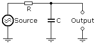
For example, when you want to convert a simple low-pass filter like this one:

The analog prototype

The Bilinear Solution

With the bilinear transformation you would get a complex algorithm like this:

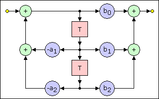
This requires 5 multiplications, 4 additions and 2 registers.

The Impulse Invariant Solution

The algorithm for a simple transformation is quite obvious:

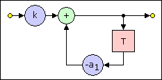
This requires 2 multiplications, 1 addition and 1 register.

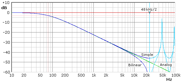
For example, with k = 0.01 and a₁ = 0.99 the algorithm is: For each sample: For the new output value take e.g. 99% of the previous output value and add 1% of the actual input value to it.

That's it. This represents a low pass filter with a time constant of 100 samples (corresponding to a corner frequency of 0.16% of the sampling frequency). For the results of this low-pass filter's bilinear and simple impulse invariant transformation see the example below.

Simple 1^st Order Analog Filters

The transfer function of a single pole / single zero analog filter is:

H(ω) =   d0 + d1 · jω  c0 + c1 · jω

The transfer function of a single pole / single zero digital filter is:

H(z) =   b0 + b1 · z-1  a0 + a1 · z-1

Usually a₀ is normalized to 1 so that the digital process looks like this:

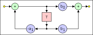
A program for this process would look like this:

Do     Output = b0 * (Input - a1 * Register) + b1 * Register     Register = Input - a1 * Register Loop

or, with the additional variable Temp:

Do     Temp = Input - a1 * Register     Output = b0 * Temp + b1 * Register     Register = Input + Temp Loop

Time Constants vs. Corner Frequencies

Often single pole filter are specified by their time constant τ instead of their corner frequency F_c. This time constant τ is calculated as follows:

τ = 1 / (2 · π · F_c)     or, vice versa:     F_c = 1 / (2 · π · τ)

Table of Coefficiensts for Some 1^st Order Filters

The coefficients for some 1^st order filters are calculated as shown in the following table.

τ is the time constant in seconds and can be derived from the corner frequency F_c, see above
G is the optional gain factor. Set G = 1 when the gain at the horizontal section of the frequency response is to be 1.
F_S is the sampling frequency in Hz

Type	1	2	3
Analog Coefficients
d0	G	0	G
d1	0	G·τ or G	τ
c0	1	1 or 1/τ	1
c1	τ	τ or 1	0
H(ω)	G 1 + τ·jω	G·τ·jω 1 + τ·jω or G·jω 1/τ + jω	G + τ·jω 1
Digital Coefficients
b0	G / (τ·FS)	G	G·τ·FS
b1	0	-G	G·(1 - b0)
a0	1
a1	b0 - 1	1 / (τ·FS) - 1	0
H(z)	G / (τ·FS) 1 + (b0 - 1)·z-1	G - G·z-1 1 + (1 / (τ·FS) - 1)·z-1	G·τ·FS + G·(1 - b0)·z-1 1

Example 1: The Simple Low-Pass Filter Mentioned Above

This sample outlines a digital low-pass filter with a time constant τ = 100 samples and no gain (i.e., G = 1). For a sample rate of 48 kHz this means τ = 100/48000 kHz = 2.08333 ms and a corner frequency  F_c = 76.394 Hz. The corresponding analog circuit could e.g. be composed of R = 2.08 kΩ and C = 1 µF.

In the formula for the digital transfer function H(z) and in the table above I use a form where the factor k does not appear. But in this case (where b₁ = 0) that's easy to convert because b₀ = k:

b₀ = 0.01
b₁ = 0
a₀ = 1
a₁ = -0.99

The resulting frequency responses are

It is obvious that in practice the difference between the ideal (analog) and the digital frequency responses can often be neglected. Also the advantages of the bilinear transformed filter, i.e., a more correct corner frequency (which is invisible here) and less susceptibility to alias frequencies will rarely matter in practice.

Example 2: RIAA Equalization Filter

The Analog Prototype

The filter parameters are given in time constants:

• 7957 µs, corresponding to a corner frequency of 20 Hz. This is a filter of type 2.
• 3180 µs, corresponding to a corner frequency of 50.05 Hz. This is a filter of type 1.
• 318 µs, corresponding to a corner frequency of 500.5 Hz. This is a filter of type 3.
• 75 µs, corresponding to a corner frequency of 2122 Hz. This is a filter of type 1.

(Note: The 20 Hz high-pass is not specified by the RIAA. It was later recommended for playback only by the EIA.)

There is no gain applied to any stage.

The analog transfer function of the RIAA equalization filter consists of three poles and two zeros and is:

H(ω) =   jω   1   1 + 0.000318·jω   1  ·   ·   ·  125.6637 + jω   1 + 0.00318·jω   1   1 + 0.000075·jω

Remark: By multiplying out this four stage transfer function it can be reduced to e.g. a two stage transfer function, one dual pole stage and one single pole / single zero stage:

H(ω) =   jω   1 + 0.000318·jω  ·  125.66 + 1.39961·jω - 0.00318·ω2   1 + 0.000075·jω

The Digital Transformation

The digital transfer function of the RIAA equalization filter is:

a) For a sample rate F_s of 48 kHz:

H(z) =   1 - z-1   0.0065513   15.264 - 14.264·z-1   0.277778  ·   ·   ·  1 - 0.99738176·z-1   1 - 0.9934486·z-1   1   1 - 0.722222·z-1

b) For a sample rate F_s of 192 kHz:

H(z) =   1 - z-1   0.0016378   61.056 - 60.056·z-1   0.0694444  ·   ·   ·  1 - 0.99934544·z-1   1 - 0.99836216·z-1   1   1 - 0.9305555·z-1

Remark: These transfer functions can also be multiplied out to form less, but more complex stages.

Note: Do not believe that because 0.99934544 is so close to 1 you could use a₁ = 1 instead. a₁ = 1 would form a perfect integrator (with a succeeding differentiator due to b₀ = 1 and b₁ = -1). Actually, for the result's precision the number of decimal places of the difference a₀- a₁ (= the difference between a₁ and 1) matters. In this case it is 0.00065456, so that the precision here is 5 decimal places. The higher the ratio F_s/F_c is, more extreme this situation becomes.

The step response for the transformation for F_s = 192 kHz has been simulated with a Visual Basic program and thus prooven to be correct.

Comparison

Now let's have a look on the resulting frequency responses of these equations and discuss them:

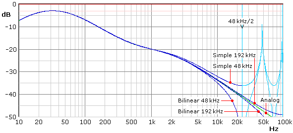
Actually 5 different frequency responses are shown. All of them are different from each other in the upper frequency range. Those marked as Simple are the ones of the transfer functions above. Those marked as Bilinear are derived from the analog prototype using bilinear transformation. All frequency responses are simulated by using my Analog-to-Digital filter conversion program AnaDigFilt.

Conclusion

The significant deviations from the ideal analog frequency response clearly point out why I wrote that simple analog to digital conversion is not always possible or useful. In this example the results with 48 kHz sampling frequency are unacceptable. This is true for the bilinear transformation but even more for the simplified impulse-invariant transformation. For 192 kHz it is significantly better, but still not better than what can easily be achieved with a non-ideal analog circuitry using available components.

In practice, the digital results could be improved by several means:

• Use upsampling, a very high upsampling frequency and downsample afterwards. This requires extreme filter efforts and/or processing power resp..
• Correct the remaining deviations by additional filter stages. Not too many of these additional stages would be required for reasonable results.
• "Cheat" by correcting the digital deviations in the previous analog preamplifier. Not much precision is necessary there to obtain a final precise frequency response.
• When it is intended to operate at different sample rates, hardly anything else than upsampling would be recommendable, probably accompanied by a very slight correction using one additional filter stage.

Though for technical reasons it may make little sense to use a digital RIAA equalizer there may be other, possibly important reasons like e.g. that its implementation is an interesting challenge or that it is a unique selling point (USP) for marketing.

Example 3: A-Weighting Filter

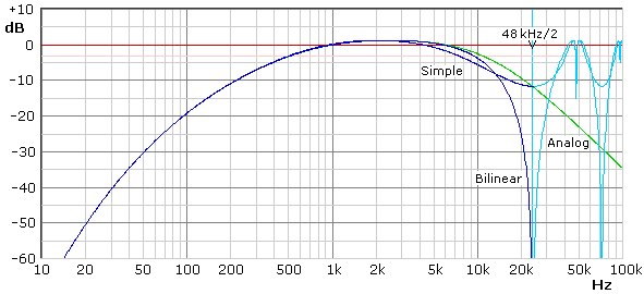
The analog transfer function forms a 6^th order filter with 4 zeros and 6 poles which can be written as 6 1^st order filter stages.

H(ω) =   0.0077263·jω   0.0077263·jω   1   1   1.305167e-5·jω   1.305167e-5·jω 2355 ·   ·   ·   ·   ·   ·  1 + 0.0077263·jω   1 + 0.0077263·jω   1 + 0.0014784·jω   1 + 2.1569e-4·jω   1 + 1.305167e-5·jω   1 + 1.305167e-5·jω

Transformed to the digital transfer function using the impulse invariant transformation results:

H(z) =   1 - z-1   1 - z-1   676.40/FS   4636.1/FS   1 - z-1   1 - z-1 2355 ·   ·   ·   ·   ·   ·  1 + (129.43/FS - 1)·z-1   1 + (129.43/FS - 1)·z-1   1 + (676.40/FS-1)·z-1   1 + (4636.1/FS-1)·z-1   1 + (76618/FS - 1)·z-1   1 + (76618/FS - 1)·z-1

A-Weighting Filter Simulation with AnaDigFilt

Both these equations cannot directly be simulated with AnaDigFilt because AnaDigFilt is prepared for a maximum of 5 filter stages only. But AnaDigFilt's filter stages are able to handle 2^nd order filters so that it is possible to combine two 1^st order filter stages each to one 2^nd order filter stage and thus to simulate the equations. In this example I combine only the first and the last pair of stages to one stage each by multiplying them out.

Analog:

H(ω) =   -5.9696E-5·ω2   2355   1   -1.7035E-10·ω2  ·   ·   ·  1 + 0.015453·jω - 5.9696E-5·ω2   1 + 0.0014784·jω   1 + 2.1569E-4·jω   1 + 2.6103E-5·jω - 1.7035E-10·ω2

Digital for F_S = 48 kHz:

H(z) =   1 - 2·z-1 + z-2   0.014092   0.096586   1 - 2·z-1 + z-2 2355 ·   ·   ·   ·  1 - 1.9946070833·z-1 + 0.9946143542·z-2   1 - 0.985908·z-1   1 - 0.903414·z-1   1 - 3.19242·z-1 + 2.54788·z-2

Comparison

As it could be expected, both frequency responses are not acceptable as weighting filters, at least not with F_S = 48 kHz. But the results are in so far interesting as both frequency responses cross each other and the "simple" frequency responses ends at F_S/2 almost exactly where it ought to. This is because the individual frequency responses of the second and the third stage (both are 1^st order low-pass filters) are slightly higher towards F_S/2 while the frequency response of the last stage (a 2^nd order high-pass filter with a corner frequency close to F_S/2) is not only significantly lower towards F_S/2, but also starts significantly earlier, visible from about 3 kHz on in the diagram.